TurboQuant: Google's Game-Changing AI Compression Algorithm
Date Published
A deep dive into how Google reduced LLM memory requirements by 6x with zero accuracy loss — and why it matters.
TL;DR
Google Research dropped TurboQuant in March 2026, and it's kind of a big deal. It compresses the key-value (KV) cache in large language models down to 3 bits without any accuracy loss. Think of it as zipping your AI's working memory — but way smarter, because the model doesn't even notice the difference.
The numbers:
6x reduction in KV cache memory
8x speed boost on attention logit computation (tested on Nvidia H100 GPUs)
Zero accuracy loss across standard benchmarks
No training or fine-tuning required — just plug it in
The Problem: Why AI Models Are So Hungry for Memory
When you're running a large language model — whether it's Gemini, GPT, Mistral, whatever — the model doesn't just load its weights and go. It maintains something called a key-value cache.
Here's the simple version: every time the model processes a token, it computes a "key" and a "value" pair. It stores these so it doesn't have to recompute them every time. It's like a cheat sheet the model keeps while writing an essay.
The problem? As context windows grow — 100K tokens, 1M tokens — that cheat sheet gets massive. We're talking tens of gigabytes just for the cache. This is why running these models costs a fortune. You need beefy GPUs with huge amounts of memory.
People have tried to compress this cache before. But every method comes with a trade-off: you compress the data, but you need extra bits to store "decompression keys" (quantization constants). It's like shrinking a zip file but having to attach a giant decoder ring. You save space, but not nearly as much as you'd hope.
TurboQuant solves this.
Architecture Overview
Here's how the whole thing fits together at a high level.

The pipeline is dead simple: PolarQuant does the heavy lifting, QJL cleans up the tiny errors, and the result goes into a compressed cache that's 6x smaller than the original.
How It Works: Two-Stage Compression
Stage 1: PolarQuant — The Heavy Lifter
PolarQuant is where the magic starts. Here's what it does:
Random rotation: Take the data vectors and randomly rotate them. This simplifies the geometry — makes the data easier to compress.
Polar coordinate conversion: Instead of using standard X, Y, Z coordinates, convert vectors to polar coordinates. Think of it like replacing "go 3 blocks east, 4 blocks north" with "go 5 blocks at 37 degrees." Same destination, but now the data has a predictable, circular pattern.
Scalar quantization: Apply standard quantization to each dimension independently. Because the data is now in polar form, you know exactly where the boundaries are — no normalization overhead.

The key insight: by rotating and converting to polar coordinates, TurboQuant eliminates the memory overhead that traditional quantization methods can't avoid. No extra bits needed for quantization constants because the pattern is already predictable.
Stage 2: QJL — The 1-Bit Error Killer
After PolarQuant does its thing, there's a tiny bit of error left. That's where QJL (Quantized Johnson-Lindenstrauss) comes in.
QJL uses a mathematical technique called the Johnson-Lindenstrauss Transform to preserve distances and relationships between data points while compressing each remaining error value to a single sign bit (+1 or -1).
One bit. That's it.

The estimator is the clever part — it balances a high-precision query with the low-precision simplified data, giving you accurate attention scores without the overhead.
Code: Implementing TurboQuant
Here's a simplified Python implementation showing the core concepts. This isn't production-ready (Google's actual implementation is more optimized), but it shows how the pieces fit together.
Core PolarQuant Implementation
1import numpy as np2from scipy.spatial.distance import cdist34class PolarQuant:5 """6 PolarQuant: Converts vectors to polar coordinates for overhead-free quantization.78 The key idea: by rotating vectors randomly and converting to polar form,9 we eliminate the need for per-block quantization constants.10 """1112 def __init__(self, n_dims: int, n_bits: int = 3):13 self.n_dims = n_dims14 self.n_bits = n_bits15 self.n_levels = 2 ** n_bits1617 # Generate a random rotation matrix (done once)18 # Uses Householder reflections for numerical stability19 self.rotation_matrix = self._generate_rotation_matrix(n_dims)2021 def _generate_rotation_matrix(self, dim: int) -> np.ndarray:22 """Generate a random orthogonal rotation matrix."""23 # Random matrix24 A = np.random.randn(dim, dim)25 # QR decomposition gives us an orthogonal matrix26 Q, _ = np.linalg.qr(A)27 return Q2829 def _to_polar(self, vector: np.ndarray) -> tuple:30 """Convert a vector to polar coordinates."""31 # For high-dim vectors, we use a recursive approach32 # This is simplified — real implementation handles dimension groups33 radius = np.linalg.norm(vector)34 if radius == 0:35 return 0.0, np.zeros(len(vector) - 1)3637 angles = []38 remaining = vector.copy()3940 for i in range(len(vector) - 1):41 r = np.linalg.norm(remaining)42 if r < 1e-10:43 angles.append(0.0)44 break45 # Compute angle with remaining dimensions46 cos_angle = remaining[0] / r47 cos_angle = np.clip(cos_angle, -1, 1)48 angles.append(np.arccos(cos_angle))49 # Project to remaining dimensions50 remaining = remaining[1:] * np.sin(angles[-1])5152 return radius, np.array(angles)5354 def _from_polar(self, radius: float, angles: np.ndarray) -> np.ndarray:55 """Convert polar coordinates back to a vector."""56 vec = np.zeros(len(angles) + 1)57 vec[0] = radius * np.cos(angles[0])5859 running_sin = np.sin(angles[0])60 for i in range(1, len(angles)):61 vec[i] = radius * running_sin * np.cos(angles[i])62 running_sin *= np.sin(angles[i])6364 vec[-1] = radius * running_sin65 return vec6667 def _scalar_quantize(self, values: np.ndarray,68 min_val: float, max_val: float) -> tuple:69 """Uniform scalar quantization."""70 step = (max_val - min_val) / (self.n_levels - 1)71 if step < 1e-10:72 indices = np.zeros(len(values), dtype=np.int32)73 return indices, min_val, step7475 indices = np.round((values - min_val) / step).astype(np.int32)76 indices = np.clip(indices, 0, self.n_levels - 1)77 return indices, min_val, step7879 def compress(self, kv_vectors: np.ndarray) -> dict:80 """81 Compress KV vectors using PolarQuant.8283 Args:84 kv_vectors: Shape (seq_len, head_dim) — the KV cache vectors8586 Returns:87 Compressed representation88 """89 # Step 1: Apply random rotation90 rotated = kv_vectors @ self.rotation_matrix9192 # Step 2: Convert to polar coordinates93 compressed = []94 metadata = []9596 for vec in rotated:97 radius, angles = self._to_polar(vec)9899 # Quantize radius (needs high precision)100 rad_idx, rad_min, rad_step = self._scalar_quantize(101 np.array([radius]), 0, np.max(np.abs(rotated))102 )103104 # Quantize angles (known distribution → no overhead!)105 ang_idx, ang_min, ang_step = self._scalar_quantize(106 angles, 0, np.pi107 )108109 compressed.append({110 'radius_idx': rad_idx[0],111 'angles_idx': ang_idx112 })113 metadata.append({114 'rad_min': rad_min, 'rad_step': rad_step,115 'ang_min': ang_min, 'ang_step': ang_step116 })117118 return {119 'compressed': compressed,120 'metadata': metadata,121 'rotation_matrix': self.rotation_matrix,122 'n_bits': self.n_bits123 }124125 def decompress(self, data: dict) -> np.ndarray:126 """Decompress back to original vector space."""127 vectors = []128129 for comp, meta in zip(data['compressed'], data['metadata']):130 # Reconstruct radius131 radius = meta['rad_min'] + comp['radius_idx'] * meta['rad_step']132133 # Reconstruct angles134 angles = meta['ang_min'] + comp['angles_idx'] * meta['ang_step']135136 # Convert from polar137 vec = self._from_polar(radius, angles)138 vectors.append(vec)139140 # Reverse rotation141 vectors = np.array(vectors)142 return vectors @ data['rotation_matrix'].T
QJL Error Correction
1class QJLErrorCorrector:2 """3 QJL: Quantized Johnson-Lindenstrauss for 1-bit error correction.45 Takes residual errors from PolarQuant and eliminates bias6 using a single sign bit per value.7 """89 def __init__(self, input_dim: int, target_dim: int):10 self.input_dim = input_dim11 self.target_dim = target_dim1213 # Random JL projection matrix14 # Scale by 1/sqrt(target_dim) for distance preservation15 self.projection = np.random.randn(input_dim, target_dim)16 self.projection /= np.sqrt(target_dim)1718 def encode_residual(self, residual: np.ndarray) -> np.ndarray:19 """20 Encode residual error using 1-bit sign quantization.2122 Args:23 residual: The small errors left after PolarQuant2425 Returns:26 1-bit encoded representation (sign bits)27 """28 # Project to lower dimension29 projected = residual @ self.projection3031 # 1-bit quantization: just the sign32 sign_bits = np.sign(projected)33 # Replace zeros randomly with +1 or -134 sign_bits[sign_bits == 0] = np.random.choice([-1, 1],35 size=np.sum(sign_bits == 0))3637 return sign_bits3839 def compute_attention_score(self, query: np.ndarray,40 compressed_key: np.ndarray,41 sign_bits: np.ndarray) -> float:42 """43 Compute attention score using the special QJL estimator.4445 The estimator combines high-precision query with low-precision46 key to produce an unbiased attention score.47 """48 # High-precision query projection49 query_proj = query @ self.projection5051 # The QJL estimator:52 # E[<q, k>] ≈ mean(q_proj * sign_bits) * ||k|| * sqrt(2/π)53 # This eliminates the bias introduced by sign quantization5455 raw_estimate = np.mean(query_proj * sign_bits)5657 # Correction factor for sign quantization bias58 # From the property: E[sign(x)] = erf(x/sqrt(2))59 # Linearized: ≈ sqrt(2/π) * x for small x60 bias_correction = np.sqrt(2 / np.pi)6162 return raw_estimate / bias_correction
Putting It Together: Full TurboQuant Pipeline
1class TurboQuant:2 """3 Full TurboQuant pipeline combining PolarQuant + QJL.45 This is the complete compression/decompression pipeline6 for KV cache quantization.7 """89 def __init__(self, head_dim: int, polar_bits: int = 2, qjl_target_dim: int = 64):10 self.head_dim = head_dim11 self.polar_quant = PolarQuant(n_dims=head_dim, n_bits=polar_bits)12 self.qjl = QJLErrorCorrector(input_dim=head_dim, target_dim=qjl_target_dim)13 self.polar_bits = polar_bits1415 # Total effective bits: ~2-3 bits for PolarQuant + 1 bit for QJL16 # vs original 32 bits → 6-10x compression17 self.effective_bits = polar_bits + 1 + (32 / head_dim) # overhead amortized1819 def compress_kv_cache(self, keys: np.ndarray, values: np.ndarray) -> dict:20 """21 Compress the full KV cache.2223 Args:24 keys: Shape (seq_len, n_heads, head_dim)25 values: Shape (seq_len, n_heads, head_dim)2627 Returns:28 Compressed KV cache representation29 """30 compressed_keys = []31 compressed_values = []32 qjl_signs_k = []33 qjl_signs_v = []3435 for head_idx in range(keys.shape[1]):36 # Compress keys with PolarQuant37 k_data = self.polar_quant.compress(keys[:, head_idx, :])3839 # Compute residual errors for QJL40 k_decompressed = self.polar_quant.decompress(k_data)41 k_residual = keys[:, head_idx, :] - k_decompressed4243 # Compress residual with QJL (1 bit)44 k_signs = self.qjl.encode_residual(k_residual)4546 compressed_keys.append(k_data)47 qjl_signs_k.append(k_signs)4849 # Same for values50 v_data = self.polar_quant.compress(values[:, head_idx, :])51 v_decompressed = self.polar_quant.decompress(v_data)52 v_residual = values[:, head_idx, :] - v_decompressed53 v_signs = self.qjl.encode_residual(v_residual)5455 compressed_values.append(v_data)56 qjl_signs_v.append(v_signs)5758 return {59 'keys': compressed_keys,60 'values': compressed_values,61 'qjl_signs_keys': qjl_signs_k,62 'qjl_signs_values': qjl_signs_v,63 'original_shape': keys.shape,64 'compression_ratio': 32 / self.effective_bits65 }6667 def compute_attention(self, query: np.ndarray,68 cache: dict) -> np.ndarray:69 """70 Compute attention scores using compressed KV cache.7172 This is where the magic happens — attention computation73 directly on compressed data with QJL-corrected scores.74 """75 seq_len, n_heads, head_dim = cache['original_shape']76 scores = np.zeros((n_heads, seq_len))7778 for head_idx in range(n_heads):79 # Decompress keys (PolarQuant only — QJL correction in score)80 k_decompressed = self.polar_quant.decompress(81 cache['keys'][head_idx]82 )8384 # Standard attention dot product on decompressed keys85 base_scores = query[head_idx] @ k_decompressed.T8687 # QJL correction: add bias-free residual correction88 qjl_signs = cache['qjl_signs_keys'][head_idx]89 qjl_correction = self.qjl.compute_attention_score(90 query[head_idx], k_decompressed, qjl_signs91 )9293 # Combine: base scores from PolarQuant + QJL correction94 scores[head_idx] = base_scores + qjl_correction9596 return scores979899# --- Usage Example ---100101# Simulate a KV cache for a small model102seq_len = 2048 # context length103n_heads = 32 # attention heads104head_dim = 128 # dimension per head105106# Generate random KV cache (in practice, this comes from the model)107keys = np.random.randn(seq_len, n_heads, head_dim).astype(np.float32)108values = np.random.randn(seq_len, n_heads, head_dim).astype(np.float32)109110original_size = keys.nbytes + values.nbytes111print(f"Original KV cache size: {original_size / 1024 / 1024:.1f} MB")112113# Compress114turbo = TurboQuant(head_dim=head_dim, polar_bits=2, qjl_target_dim=64)115compressed = turbo.compress_kv_cache(keys, values)116117# Approximate compressed size118compressed_size = sum(119 sum(arr.nbytes for arr in head_data['compressed']120 for head_data in [head_data])121 for head_data in [compressed['keys']]122) + sum(signs.nbytes for signs in compressed['qjl_signs_keys'])123124print(f"Compressed size: ~{compressed_size / 1024 / 1024:.1f} MB")125print(f"Compression ratio: {compressed['compression_ratio']:.1f}x")126127# Compute attention on compressed cache128query = np.random.randn(n_heads, head_dim).astype(np.float32)129scores = turbo.compute_attention(query, compressed)130print(f"Attention scores shape: {scores.shape}")131print("✓ TurboQuant pipeline complete")
Data Flow Architecture
Here's how data flows through the entire system during inference:

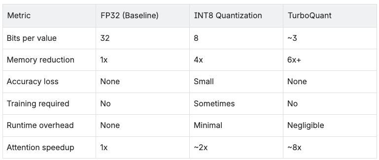
Performance Comparison
Let's put the numbers in perspective:

Where TurboQuant Fits in the LLM Stack

TurboQuant lives in the Memory Layer, specifically managing the KV cache. It doesn't touch model weights or activations — just the cache that grows with sequence length.
Market Impact: The Ripple Effect
The day Google announced TurboQuant, memory chip stocks took a hit:
Samsung: Down ~3%
Micron: Down ~5%
SK Hynix: Down ~4%
The market's logic: if models need 6x less memory, who's buying all these chips?
But analysts see it differently. Morgan Stanley's take: more intense computing, not less demand. Lower inference costs → more AI adoption → more total compute needed. The same thing happened when compression algorithms improved internet bandwidth — people didn't use less internet, they used more.
Forbes theorized that reducing hardware barriers could actually accelerate localized AI projects, paradoxically driving up total long-term chip consumption.
The community reaction was fast:
Ported to llama.cpp within 24 hours
Ported to MLX (Apple Silicon) within 48 hours
Reddit calling it "the democratization of local AI"
What This Means for You
If you're running LLMs at scale: Expect inference costs to drop 30-50%. This isn't a maybe — it's a when. Once TurboQuant is integrated into popular inference frameworks, it's just a flag you flip.
If you're building on-device AI: TurboQuant makes larger models viable on constrained hardware. Running a 13B model on a phone? Getting closer every day.
If you're in the chip business: The narrative shifts from "more memory" to "smarter memory." Companies that adapt win. Companies that don't, well...
If you're a researcher: The paper is at arxiv.org/abs/2504.19874. Being presented at ICLR 2026. The code approach is elegant — worth studying even if you never use TurboQuant itself.
Sources
Google Research Blog: turboquant-redefining-ai-efficiency-with-extreme-compression
Paper: arxiv.org/abs/2504.19874
Tom's Hardware: turboquant-compresses-llm-kv-caches-to-3-bits
TechCrunch: google-turboquant-ai-memory-compression
VentureBeat: turboquant-algorithm-speeds-up-ai-memory-8x
Written for people who want to understand the how, not just the what.